Time Series
A time series is a list of observations collected sequentially, usually over time. Common time series subjects are stock prices, population levels, product sales, rainfall, and temperature. It’s assumed that the observations are taken at uniform time intervals, such as every day, month, or year. Not all time series occur over time. For example, a list of diameters taken at every meter along a telephone cable is a legitimate time series.
Observations in a time series are often sequentially dependent. For example, population levels in the future often depend on levels at present and in the past. The goal of time series analysis is to model the nature of these dependencies, which in turn allows you to predict, or forecast, observations that have not yet been made.
The Time Series Plot procedure is used to create a time series plot for one or more variables. The values of the variables are plotted in case order. Options include line plot, connected symbols plot, connected digits plot, vertical line plot, and flexible axis labels.
The Autocorrelation Plotprocedure is used to create an autocorrelation plot for a specified variable.
Approximate 95% confidence intervals are included.
The Partial Autocorrelation Plot procedure is used to create a partial autocorrelation plot for a specified variable. Approximate 95% confidence intervals are included.
The Cross Correlation procedure is used to create a cross correlation plot for two variables.
The Moving Averages procedure is used to compute forecasts for time series data. Both single and double moving averages techniques are available. Use single moving averages when there is no trend in the time series data. Use double moving averages when there is a trend in the data.
The Exponential Smoothing procedure computes forecasts for time series data using exponentially weighted averages. Five different models are available to fit no trend data, trend data, and trend with seasonal data. Results include model diagnostics, forecast table, forecast plot, residuals plot, save residuals.
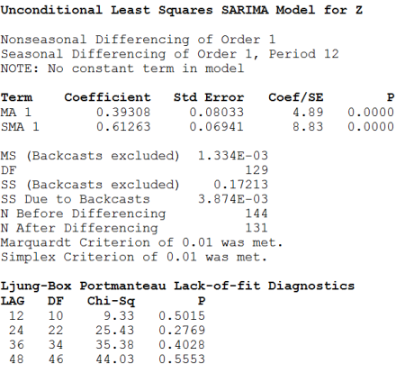
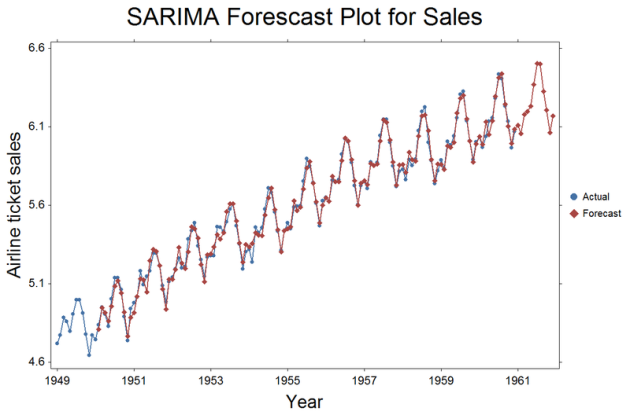
The SARIMA procedure allows you to fit a variety of models to data, including both nonseasonal and multiplicative, and nonmultiplicative seasonal models. SARIMA stands for Seasonal AutoRegressive Integrated Moving Average. It’s a procedure for modeling time series popularized by Box and Jenkins (1976). MA and AR terms need not be sequential, so nonsignificant terms don’t need to be included in the model. Results includes parameter estimates, approximate significance levels, and several statistics useful for diagnosing model fit. You can also obtain forecasts with confidence intervals. You can save fitted values and residuals to evaluate model adequacy. Estimation is based on unconditional least squares, also known as the backcasting method.
Example Reports and Plots